GraphQL Static Analysis Example

In this blog post I want to get much more specific with a detailed example of how to do GraphQL Static Query Analysis.

This article is Part 3 in a 7-Part Series. (7 posts to date, more planned)

• Part 1 - Why does GraphQL need cost analysis?
• Part 2 - Methods of GraphQL Cost Analysis
• Part 3 - This Article
• Part 4 - Survey of GraphQL Cost Analysis in 2021: Public Endpoints and Open Source Libraries
• Part 5 - Survey of GraphQL Cost Analysis in 2021: Products and Academia
• Part 6 - Introducing: GraphQL Cost Directives Specification
• Part 7 - API Days Interface: GraphQL Cost Directives Specification

I think this post works really well as a short video:

---

Background

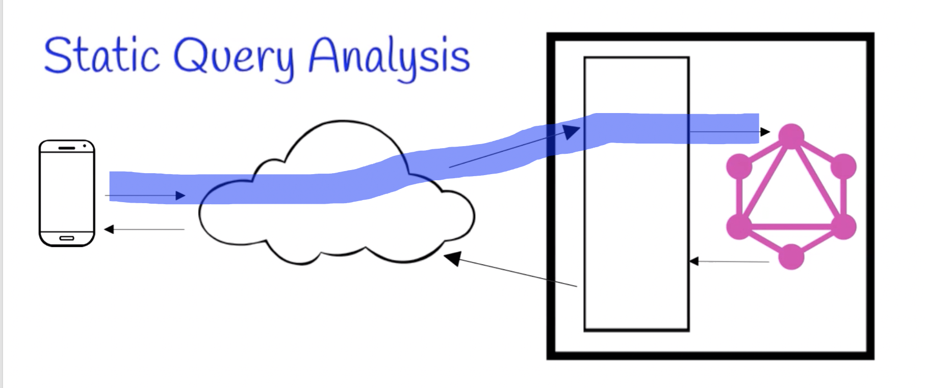
In this post we’re discussing Static Query Analysis in particular. For a review of how it compares to the other methods and where it is run, please refer to the post defining the different methods of GraphQL cost analysis. For a motivation of why this is important, see Why GraphQL Cost Analysis is important.

Inputs

GraphQL static query analysis requires two inputs:

• A GraphQL schema
• A GraphQL input - query, mutation, or subscription

Here’s part of a GraphQL schema for a fictional bank. It describes transactions, lists of transactions, and accounts that have those lists.

""" The top level queries that are supported """
type Query {
  customer (id: ID!): Customer
  customers (first: Int, last: Int, after: ID, before: ID): CustomerConnection
  account (id: ID!): Account
  accounts (first: Int, last: Int, after: ID, before: ID): AccountConnection
}

The second thing we need is a query to analyze against that schema.

query fetchPage {
  account(id: "ab1035") {
    name
    transactions(last: 5) {
      pageInfo {
        hasNextPage
      }
      edges {
        cursor
        node {
          date
          amount
        }
      }
    }
  }
}

The client wants to show a mobile screen for a bank account with the last 5 transactions. So the query asks for:

• The account name — with name
• Whether there are earlier transactions which would require a “Next Page” button — with hasNextPage
• The dates and amounts for the recent transactions — with date and amount

Static Query Analysis

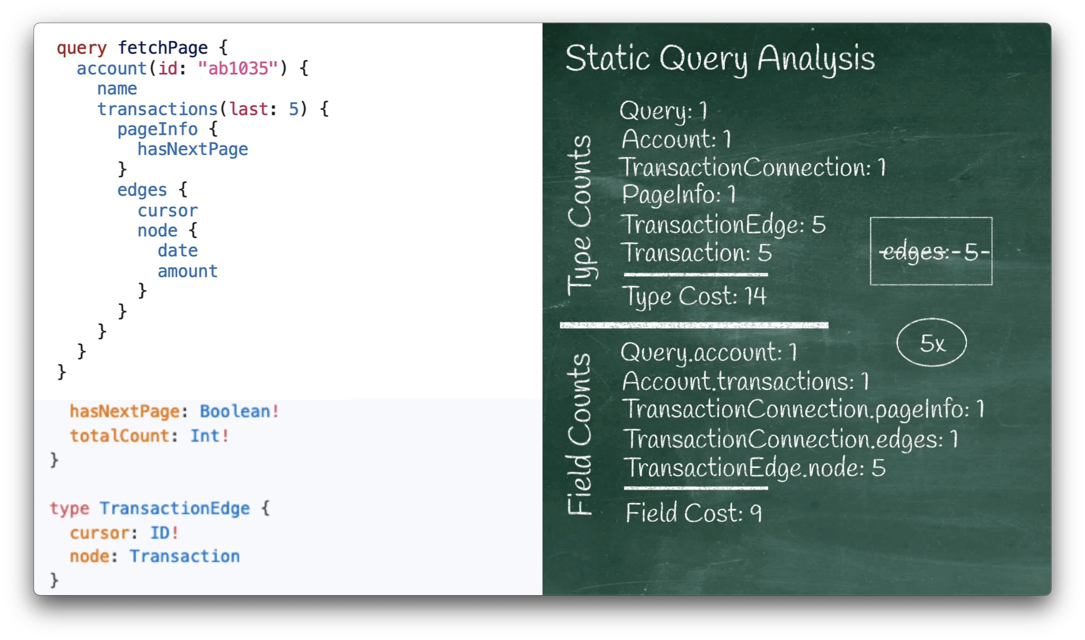
We run through the query line by line, from top to bottom, while keeping a pointer to the relevant part of the schema at all times. As we go, we keep track of counts of the GraphQL types and fields.

• For Type Counts, we’re keeping track of how many times at most this type might be returned in the response.
• For Field Counts, we’re keeping track of how many times at most the resolver function for this field might be called in the GraphQL execution engine.

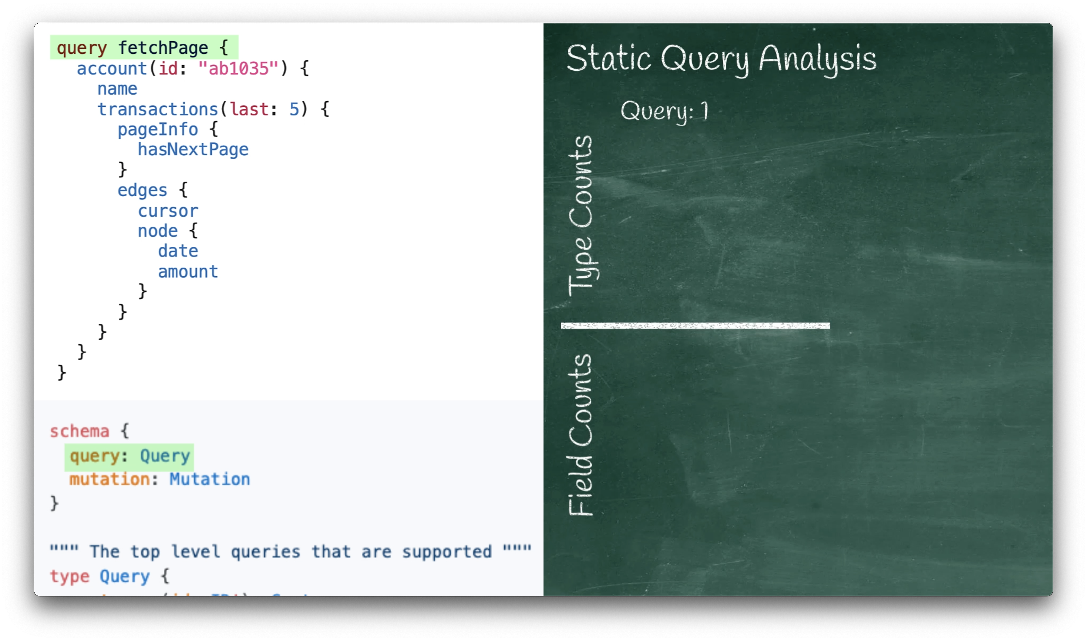
We start with the first line:

query fetchPage {

With the keyword query in the input, we look in the schema for the ‘query root operation type’:

schema {
  query: Query
  mutation: Mutation
}

… and from there we find the Query type:

type Query {
   ...
}

At this point, we can add 1 to our Query count:

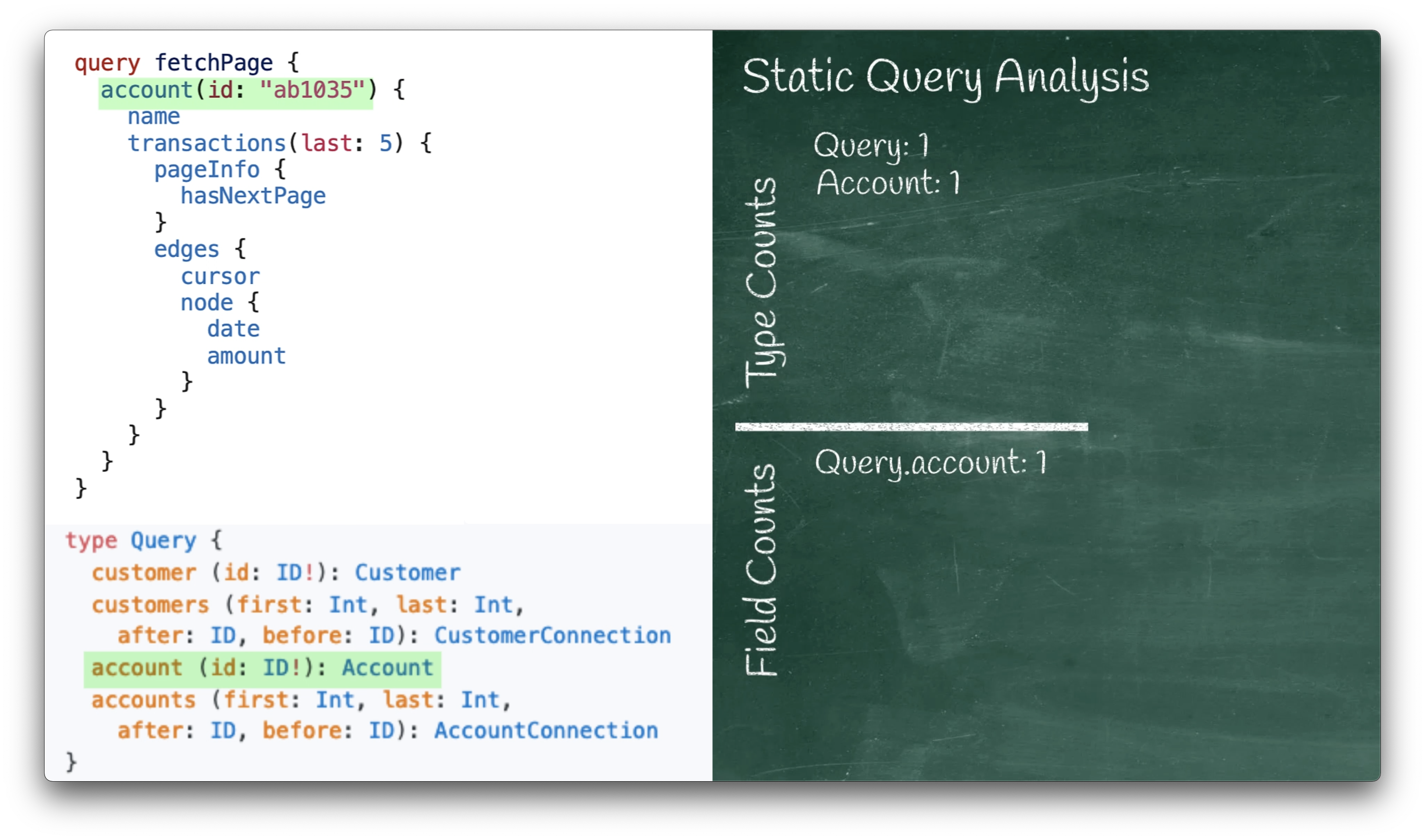
The next line in the query has an account:

  account(id: "ab1035") {

This corresponds to the Query.account field in our schema:

type Query {
  ...
  account (id: ID!): Account
  ...
}

When this field is encountered in the GraphQL execution engine, it would run the Query.account resolver function, so we add 1 to our field count for Query.account. When the GraphQL execution engine runs that resolver function, it would return either null or an object of type Account, so we increment our type count for Account.

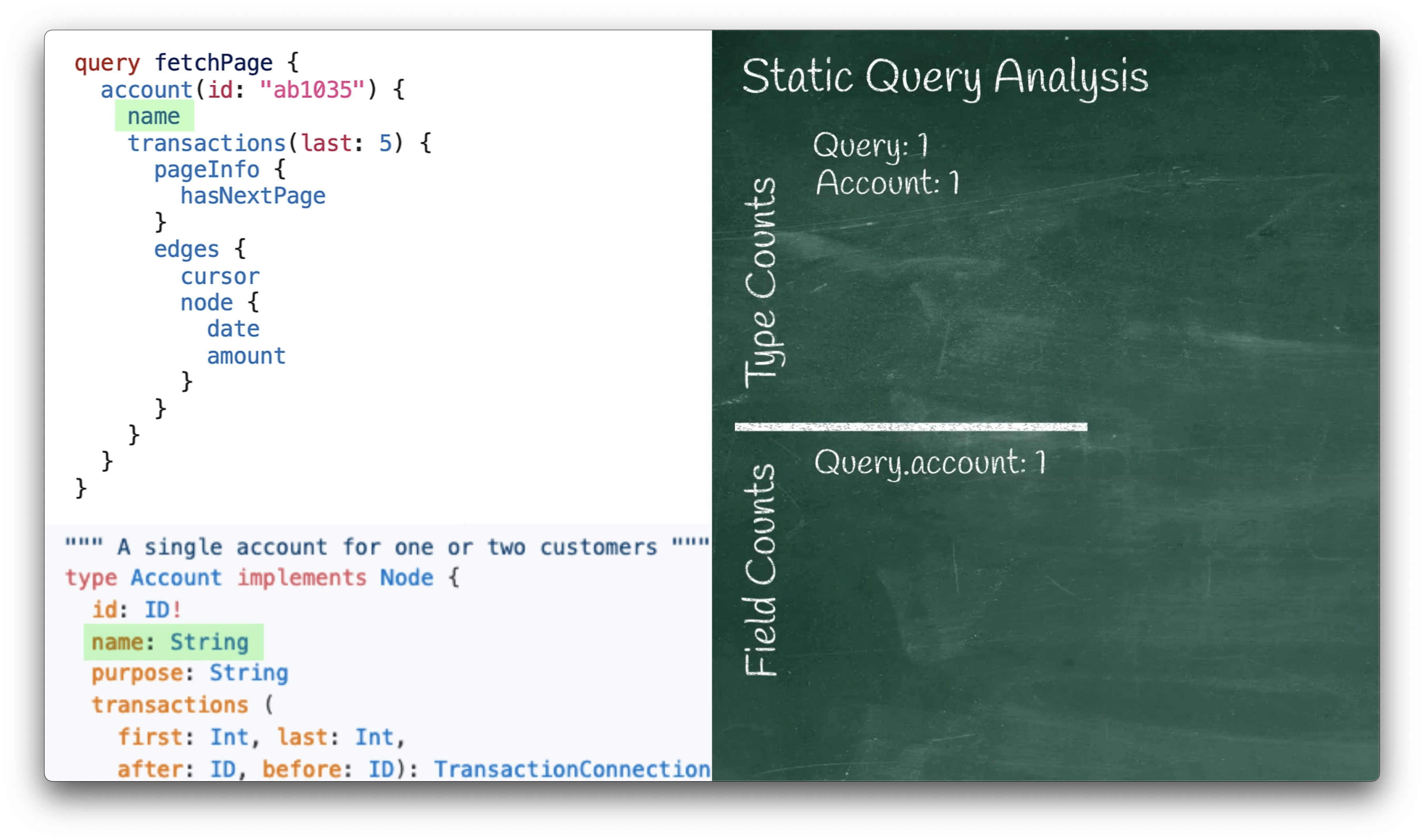
The next line in the query has a name:

    name

This corresponds to the ‘Account.name’ field in our schema:

type Account {
  ...
  name: String
  ...
}

Since name is of type String, which is a simple scalar type, we skip it in our analysis. By default we’ll assume that any scalar value is just a quick lookup within the object already retrieved by the resolver function that returned the enclosing type. For example, one resolver will often retrieve a database record as a JSON object, and then sub-fields will merely retrieve sub-values from that JSON object, which doesn’t even have to query the database again. If so, then the execution engine can handle this lookup quickly, and it’s not worth counting.

Note that this is configurable, since you might have a scalar type that is expensive to compute, such as:

type LifeTheUniverseAndEverything {
    question: String!
    answer: Int!
}

In our case, name is simple to pull from the account record, so we stick with the default, which means that our analysis does not update any type or field counts:

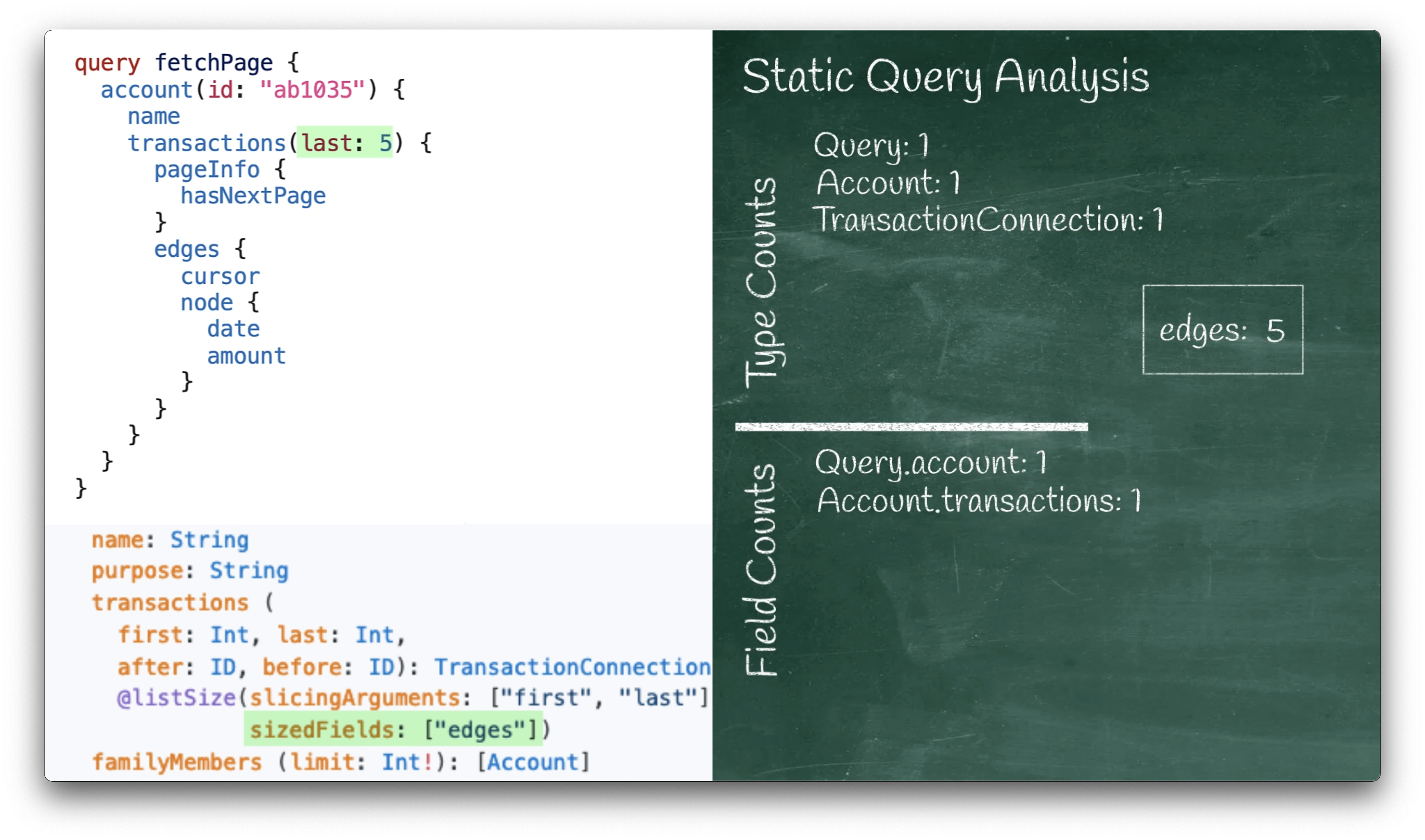
The next line in the query asks for a list of transactions:

    transactions(last: 5) {

This corresponds to the Account.transactions field in our schema:

type Account {
  ...
  transactions (
    first: Int, last: Int,
    after: ID, before: ID): TransactionConnection
    @listSize(slicingArguments: ["first", "last"]
              sizedFields: ["edges"])
  ...
}

Part of this looks familiar: When this field is encountered by the GraphQL execution engine, we expect it to run the Account.transactions resolver function, so we add 1 to our field count for Account.transactions. That resolver function returns either null or an object of type TransactionConnection, so we also increment our type count for TransactionConnection.

Another part of this is new: There is extra information about this field in the schema. Each one of the slicingArguments tells us that its integer value gives an upper bound on the size of an upcoming list. So we take the 5 from the last argument and record it for future reference.

The single member of the sizedFields list is edges, which tells us that we’ll apply this new list size of 5 only when we get to the edges field. We add that to our recorded note, and ignore it until we later see edges.

Note: Using first and last as integer arguments to bound the size of a returned list which is provided by an edges sub-field is a very standard pattern for GraphQL, used by both GraphQL pagination and the Relay connections standard.

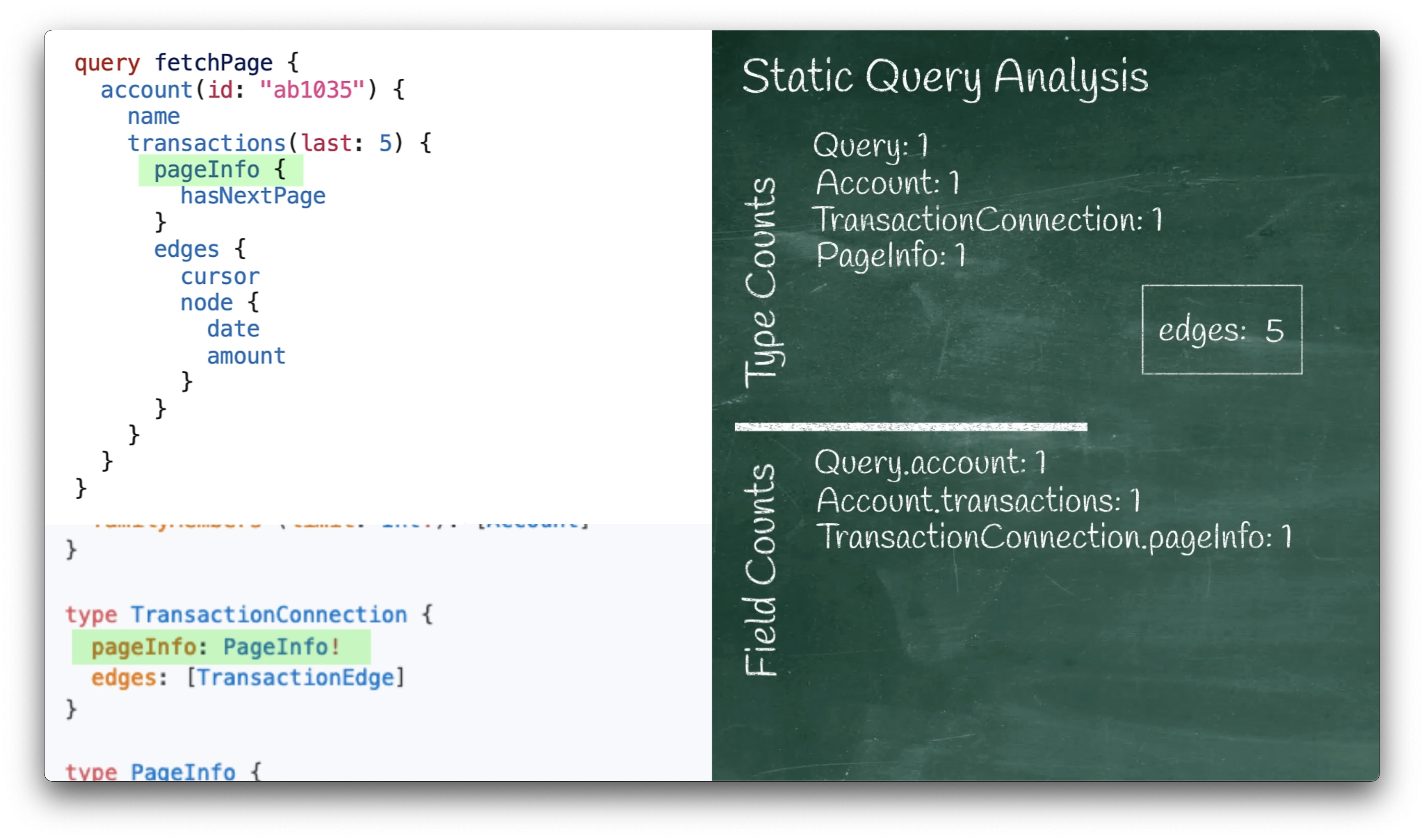
The next couple of lines are simple enough, a pageInfo followed by a hasNextPage:

      pageInfo {
        hasNextPage
      }

This corresponds to the TransactionConnection.pageInfo and PageInfo.hasNextPage fields in our schema:

type PageInfo {
  hasNextPage: Boolean!
  totalCount: Int!
}

type TransactionConnection {
  pageInfo: PageInfo!
  edges: [TransactionEdge]
}

PageInfo adds both a field and a type to our counts, and hasNextPage is a scalar, so we skip it like we did with the string earlier.

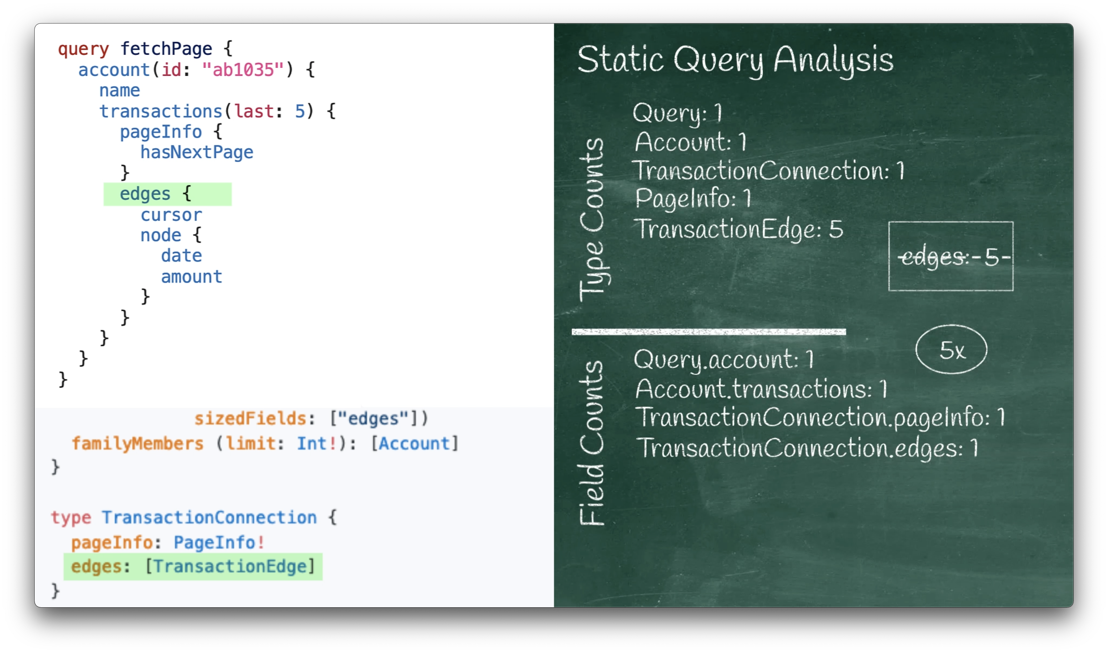
When we get to edges it’s time to apply our note that we had saved for later.

      edges {

It’s obvious that we need to run that resolver function once, but it returns a list. While a base GraphQL schema doesn’t bound that list size, our extra directives did. Remember the 5 from the last argument that we wrote down would apply to the edges field? Now we use that fact to know that at most 5 TransactionEdge types are returned from TransactionConnection.edges.

type TransactionConnection {
  ...
  edges: [TransactionEdge]
}

As we record those counts and move into the edges part of our graph, we cross out our extra information, while we make a new note that everything in this sub-tree might be run on 5 different objects.

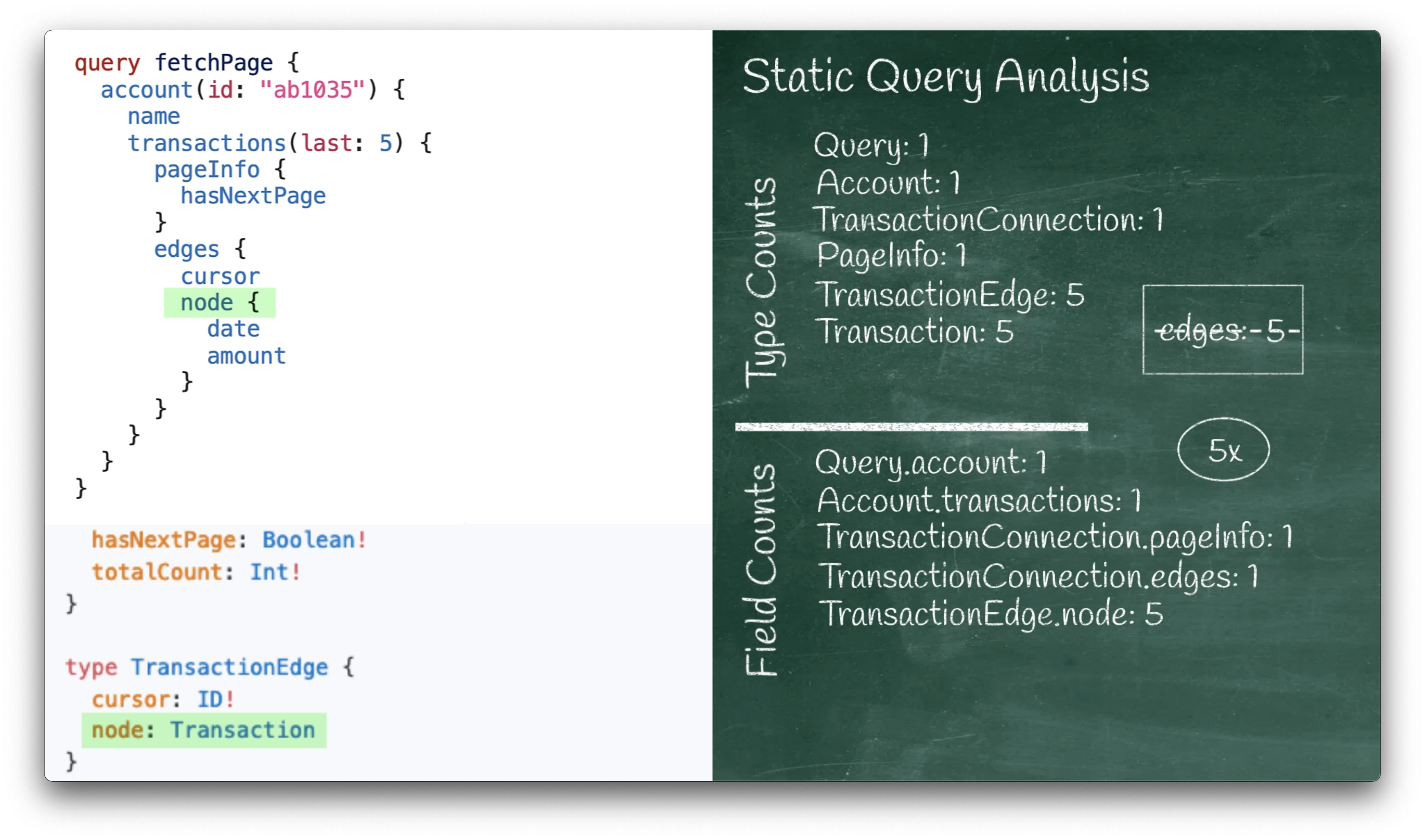
The next line in the query requests a cursor value:

        cursor

This corresponds to the ‘TransactionEdge.cursor’ field in our schema:

type TransactionEdge {
  cursor: ID!
  ...
}

Since cursor is defined to be a scalar type (ID), we skip it by default just like we did with the String name and the Boolean hasNextPage.

The last non-scalar line in our query is node:

        node {

This corresponds to the TransactionEdge.node field in our schema:

type TransactionEdge {
  ...
  node: Transaction
}

We run our TransactionEdge.node once per object, but how many objects might we run it on? Remember that we wrote that we would be running this sub-tree at most 5 times, due to our upper bound of the list size. That means that we will run TransactionEdge.node at most 5 times.

Each of those 5 times returns a Transaction so we might get up to 5 of objects of type Transaction.

Finally we search through the rest of the query, finding two more scalars:

          date
          amount

This corresponds to the Transaction.date and Transaction.amount fields in our schema:

type Transaction {
  ...
  date: String
  amount: Float!
  ...
}

Since both have scalar types, we don’t count either one of them, and that brings us to the end of the input query.

All that’s left is to take a weighted sum of these counts. By default all the weights are 1, so our weighted sum is just a simple sum, and gives us a type cost of 14 and a field cost of 9.

If we wanted to say that some types or fields were more costly than others, then we could instead let the counts affect the cost in a non-uniform manner to accurately reflect the transaction’s cost or expense, according to the internals of our actual GraphQL server.

Both costs are important:

• Type cost roughly corresponds to how much data this query might produce.
• Field cost corresponds to how much work might need to be done to produce that data.

Once we have these calculated costs, we can use them on a proxy or in middleware running with our GraphQL server for threat protection, monetization, and rate limiting.

When we evaluate the usefulness of GraphQL Static Query Analysis:

• The main drawback is that it calculates upper bounds instead of exact cost metrics.
• The main advantage is that it is calculated without even starting your GraphQL execution engine, which means that there was no risk to your databases and other backend systems.

I hope this concrete example gives you a good sense of what to expect from Static Query Analysis, and how to do it yourself.